Line Follower Bot

Line follower is an autonomous robot that follows a line, either a black line on white surface or vise-versa. Robot must be able to detect particular line and keep following it.

For special situations such as cross overs where robot can have more than one path which can be followed, predefined path must be followed by the robot.

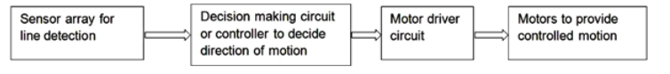
The main electronics/mechanical components that will be used in making this line follower robot are IR sensors, motor-drivers and microcontroller.

BLOCK DIAGRAM
SENSORS
PID ALGORITHM
LINE FOLLOWER BOTS IN ACTION (LF 2016, IIT Bombay)

BLOCK DIAGRAM

Block Diagram

SENSORS

Sensors are required to detect position of the line to be followed with respect to the robot’s position. Most widely used sensors for the line follower robot are photosensors. They are based on the basic observation that “the white surface reflects the light and the black surface absorbs it”.IR sensors are used preferably to avoid interference with visible light.

Sensor circuit contains an emitter and a detector. Photodetector is used to detect the intensity of light reflected. The corresponding analog voltage is induced based on the intensity of reflected light.

The analog voltage is converted to digital voltage by ADC and compared with a certain threshold to generate a logic ‘1’ or ‘0’ which is used by the controller.

The main algorithm behind making the Line Follower Bot is the PID Algorithm, which is described in detail below.

PID ALGORITHM

First off, let’s start with an example. You want to build a system to make a car run at some constant speed, say 40 Km/h. What could possibly be done? Well, you could fix the accelerator at some carefully calibrated position. But hey, this wouldn’t work so well in the long run, would it? The calibration can go off with time, and it most certainly won’t work on slopes. What could possibly be done?

Yep! We need to continuously monitor the car’s speed and “press the accelerator more if it is going too slow and press the accelerator less if it is going too fast. If it is going too fast even after the accelerator is completely released, then press the brakes.” Now that can be called a control loop, where you monitor the output and feed some of it it to the input.

Well, that was a bit vague. If the car was going at more than the set speed, do you release the accelerator completely? Of if it’s going too slow, you shouldn’t slam the accelerator, should you?

So let us define the Process Variable as the current speed, the Set Point as the value the Process variable is required to maintain, and the Error as the difference between Set Point and Process variable.

$$ e = SP - PV $$

So the error in this case would be 40 – <Current speed of the car>. Clearly, e has to be minimised.

Let’s say we press the accelerator by an amount u(t). Press the accelerator if u is positive, and brakes if u is negative.

Further, let’s say u(t) is dependent on e as per the following relation.

$$ U(t) = K_p*e $$

Where Kp is some proportionality constant.

This will obviously minimise error. But hey, doesn’t this equation remind you of something?

$$ F= K * (x_0 – x) $$

Well, as the analogy suggests, there is going to be an inherent oscillating tendency to the system. The speed of the car tends to increase and decrease over time. Hence we need to do something to dampen the oscillation. Following the analogy of the pendulum, the damping should be proportional to the rate of change of the Process Variable.

Let us now modify the expression for u(t).

$$ U(t) = K_p*e + K_d * \frac{de}{dt} $$

Well, that was taken care of. But hey, there is a gaping hole here! The equation suggests that if the error is zero for a few seconds, then neither the accelerator nor brake has to be pressed – Hardly the case!

To compensate for this, we add an integral term, which takes into account the history of the system and provides the necessary ‘offset’ for u(t).

$$ U(t) = K_p*e + K_i*\int_0^t e dt + K_d*\frac{de}{dt} $$

If the car is mostly running at less than the targeted speed, the integral term takes a positive value, and vice versa. It provides the necessary ‘offset’ to u(t).

Needless to say, all these parameters K_p , K_i and K_d have optimal values. There are many methods to figure out their values, including self-tuning algorithms. But more often than not, it is convenient to manually tune their values for small applications rather than incorporate a complex tuning algorithm.

Here is a sample pseudo-code which implements the PID algorithm in practice.

Initialise I and e_previous as 0
loop{
	e = error();     \\error() is a pre defined function
	D = (e - e_previous)/0.01;
	I = I + 0.01 * e;
	u = Kp * e + Ki * I + Kd * D;
	e_previous = e;
	process(u);     \\press accelerator/brake according to u
	delay(10);    \\10 millisecond	
}

The PID algorithm has loads of applications – starting from line followers and quadcopters to industrial robotic arms.

It is usually best to first tweak the value of K_p, keeping the other two zero, then K_i and finally K_d.

Now, coming to the technicalities of the code- The code can either be written in AVR or in Arduino. AVR is certainly more difficult to implement than Arduino.

Link to AVR tutorial
Link to Arduino tutorial

Here’s an awesome Line Follower bot in action.